Examples using the module graph3.asy of the Asymptote drawing
software
graph3-fig001
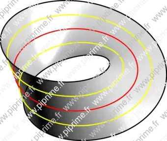
A Möbius strip of half-width with midcircle of radius
and at height can be represented parametrically by :
for in and in . In this parametrization, the Möbius strip is therefore a cubic surface with equation
Source
Show graph3/fig0010.asy on Github.
Generated with Asymptote 3.00-0.
Categories : Examples 3D | Graph3.asy
Tags : #Graph (3D) | #Surface | #Level set (3D)
import graph3;
ngraph=200;
size(12cm,0);
currentprojection=orthographic(-4,-4,5);

real x(real t), y(real t), z(real t);

real R=2;
void xyzset(real s){
  x=new real(real t){return (R+s*cos(t/2))*cos(t);};
  y=new real(real t){return (R+s*cos(t/2))*sin(t);};
  z=new real(real t){return s*sin(t/2);};
}


int n=ngraph;
real w=1;
real s=-w, st=2w/n;
path3 p;
triple[][] ts;
for (int i=0; i <= n; ++i) {
  xyzset(s);
  p=graph(x,y,z,0,2pi);

  ts.push(new triple[] {});
  for (int j=0; j <= ngraph; ++j) {
    ts[i].push(point(p,j));
  }
  s += st;
}

pen[] pens={black, yellow, red, yellow, black};
draw(surface(ts, new bool[][]{}), lightgrey);
for (int i=0; i <= 4; ++i) {
  xyzset(-w+i*w/2);
  draw(graph(x,y,z,0,2pi), 2bp+pens[i]);
}
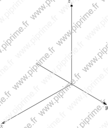
graph3-fig002
Show graph3/fig0020.asy on Github.
Generated with Asymptote 3.00-0.
Categories : Examples 3D | Graph3.asy
Tags : #Graph (3D) | #Axis (3D)
import graph3;

size(8cm,0);
currentprojection=orthographic(1,1,1);

limits((0,-2,0),(2,2,2));

xaxis3("$x$", OutTicks());
yaxis3("$y$", OutTicks());
zaxis3("$z$", OutTicks());
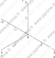
graph3-fig003
Show graph3/fig0030.asy on Github.
Generated with Asymptote 3.00-0.
Categories : Examples 3D | Graph3.asy
Tags : #Graph (3D) | #Axis (3D)
import graph3;

size(8cm,0,IgnoreAspect);
currentprojection=orthographic(1,1,1);

limits((0,-2,0), (2,2,2));

axes3("$x$","$y$","$z$",Arrow3);
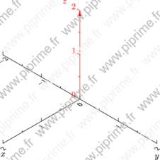
graph3-fig004
Show graph3/fig0040.asy on Github.
Generated with Asymptote 3.00-0.
Categories : Examples 3D | Graph3.asy
Tags : #Graph (3D) | #Axis (3D)
import graph3;

size(8cm,0);
currentprojection=orthographic(1,1,1);

defaultpen(overwrite(SuppressQuiet));

limits((0,-2,0),(2,2,2));

xaxis3("$x$", InTicks(XY()*Label));
yaxis3("$y$", InTicks(XY()*Label));
zaxis3("$z$", OutTicks, p=red, arrow=Arrow3);
graph3-fig005
Show graph3/fig0050.asy on Github.
Generated with Asymptote 3.00-0.
Categories : Examples 3D | Graph3.asy
Tags : #Graph (3D) | #Axis (3D)
import graph3;

size(6cm,0);
currentprojection=orthographic(1,1,1);

limits((-2,-2,0),(0,2,2));

xaxis3(Label("$x$",MidPoint), OutTicks());
yaxis3("$y$", InTicks());
zaxis3("$z$",XYEquals(-2,0), OutTicks());
graph3-fig006
Show graph3/fig0060.asy on Github.
Generated with Asymptote 3.00-0.
Categories : Examples 3D | Graph3.asy
Tags : #Graph (3D) | #Axis (3D)
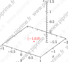
import graph3;
usepackage("icomma");

size(8cm,0);
currentprojection=orthographic(1.5,1,1);

limits((-2,-1,-.5), (0,1,1.5));

xaxis3("$x$",
       Bounds(Both,Value),
       OutTicks(endlabel=false));

yaxis3("$y$",
       Bounds(Both,Value),
       OutTicks(Step=.5,step=.25));

zaxis3("$z$", XYEquals(-2,0), InOutTicks(Label(align=Y-X)));

dot(Label("",align=Z), (-1,0,0), red);
graph3-fig007
Show graph3/fig0070.asy on Github.
Generated with Asymptote 3.00-0.
Categories : Examples 3D | Graph3.asy
Tags : #Graph (3D) | #Axis (3D) | #Triple
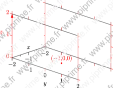
import graph3;

size(8cm,0);
currentprojection=orthographic(1,1,0.5);
limits((-2,-2,0),(0,2,2));

xaxis3(Label("$x$",align=Z),
       Bounds(Min,Min),
       OutTicks(endlabel=false,Step=1,step=0.5));

yaxis3("$y$", Bounds(),
       OutTicks(pTick=0.8*red, ptick=lightgrey));

zaxis3("$z$", Bounds(),
       OutTicks, p=red, arrow=Arrow3);

dot(Label("",align=Z), (-1,0,0), red);
graph3-fig008
Show graph3/fig0080.asy on Github.
Generated with Asymptote 3.00-0.
Categories : Examples 3D | Graph3.asy
Tags : #Graph (3D) | #Surface | #Level set (3D) | #Contour | #Function (implicit)
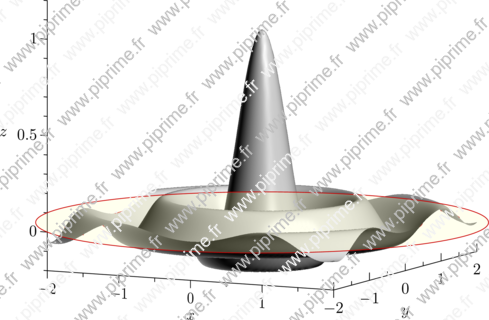
// Adapted from the documentation of Asymptote.
import graph3;
import contour;
texpreamble("\usepackage{icomma}");

size3(12cm, 12cm, 8cm, IgnoreAspect);

real sinc(pair z) {
  real r=2pi*abs(z);
  return r != 0 ? sin(r)/r : 1;
}

limits((-2, -2, -0.2), (2, 2, 1.2));
currentprojection=orthographic(1, -2, 0.5);

xaxis3(rotate(90, X)*"$x$",
       Bounds(Min, Min),
       OutTicks(rotate(90, X)*Label, endlabel=false));

yaxis3("$y$", Bounds(Max, Min), InTicks(Label));
zaxis3("$z$", Bounds(Min, Min), OutTicks());

draw(lift(sinc, contour(sinc, (-2, -2), (2, 2), new real[] {0})), bp+0.8*red);
draw(surface(sinc, (-2, -2), (2, 2), nx=100, Spline), lightgray);

draw(scale3(2*sqrt(2))*unitdisk, paleyellow+opacity(0.25), nolight);
draw(scale3(2*sqrt(2))*unitcircle3, 0.8*red);
graph3-fig009
Show graph3/fig0090.asy on Github.
Generated with Asymptote 3.00-0.
Categories : Examples 3D | Graph3.asy
Tags : #Graph (3D) | #Surface | #Level set (3D) | #Contour | #Function (implicit) | #Palette
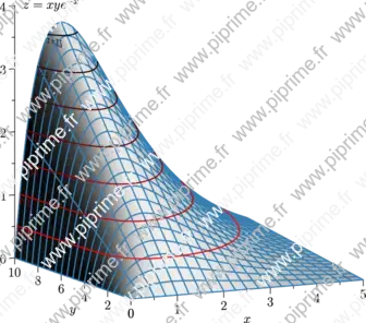
size(12cm,0,false);
import graph3;
import contour;
import palette;

texpreamble("\usepackage{icomma}");

real f(pair z) {return z.x*z.y*exp(-z.x);}

currentprojection=orthographic(-2.5,-5,1);

draw(surface(f,(0,0),(5,10),20,Spline),palegray,bp+rgb(0.2,0.5,0.7));

scale(true);

xaxis3(Label("$x$",MidPoint),OutTicks());
yaxis3(Label("$y$",MidPoint),OutTicks(Step=2));
zaxis3(Label("$z=xye^{-x}$",Relative(1),align=2E),Bounds(Min,Max),OutTicks);

real[] datumz={0.5,1,1.5,2,2.5,3,3.5};

Label[] L=sequence(new Label(int i) {
    return YZ()*(Label(format("$z=%g$",datumz[i]),
                       align=2currentprojection.vector()-1.5Z,Relative(1)));
  },datumz.length);

pen fontsize=bp+fontsize(10);
draw(L,lift(f,contour(f,(0,0),(5,10),datumz)),
     palette(datumz,Gradient(fontsize+red,fontsize+black)));
graph3-fig010
Show graph3/fig0100.asy on Github.
Generated with Asymptote 3.00-0.
Categories : Examples 3D | Graph3.asy
Tags : #Graph | #Contour | #Function (implicit) | #Palette | #Axis | #Array
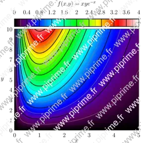
// From documentation of Asymptote
import graph;
import palette;
import contour;
texpreamble("\usepackage{icomma}");

size(10cm,10cm,IgnoreAspect);

pair a=(0,0);
pair b=(5,10);

real fz(pair z) {
  return z.x*z.y*exp(-z.x);
}
real f(real x, real y) {return fz((x,y));}

int N=200;
int Divs=10;
int divs=2;

defaultpen(1bp);
pen Tickpen=black;
pen tickpen=gray+0.5*linewidth(currentpen);
pen[] Palette=BWRainbow();

scale(false);

bounds range=image(f,Automatic,a,b,N,Palette);

xaxis("$x$",BottomTop,LeftTicks(pTick=grey, ptick=invisible, extend=true));
yaxis("$y$",LeftRight,RightTicks(pTick=grey, ptick=invisible, extend=true));

// Major contours
real[] Cvals;
Cvals=sequence(11)/10 * (range.max-range.min) + range.min;
draw(contour(f,a,b,Cvals,N,operator ..),Tickpen);

// Minor contours
real[] cvals;
real[] sumarr=sequence(1,divs-1)/divs * (range.max-range.min)/Divs;
for (int ival=0; ival < Cvals.length-1; ++ival)
    cvals.append(Cvals[ival]+sumarr);
draw(contour(f,a,b,cvals,N,operator ..),tickpen);

palette("$f(x,y)=xye^{-x}$",range,point(NW)+(0,1),point(NE)+(0,0.25),Top,Palette,
        PaletteTicks(N=Divs,n=divs,Tickpen,tickpen));
graph3-fig011
Show graph3/fig0110.asy on Github.
Generated with Asymptote 3.00-0.
Categories : Examples 3D | Graph3.asy
Tags : #Graph (3D) | #Surface | #Level set (3D) | #Contour | #Function (implicit) | #Palette | #Projection (3D) | #Axis (3D) | #Label (3D) | #Shading (3D) | #Shading
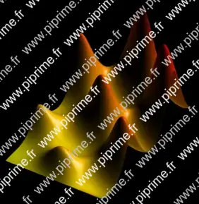
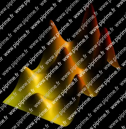
import graph3;
import palette;
import contour;
size(14cm,0);
currentprojection=orthographic(-1,-1.5,0.75);
currentlight=(-1,0,5);

real a=1, b=1;
real f(pair z) { return a*(6+sin(z.x/b)+sin(z.y/b));}
real g(pair z){return f(z)-6a;}

// The axes
limits((0,0,4a),(14,14,8a));
xaxis3(Label("$x$",MidPoint),OutTicks());
yaxis3(Label("$y$",MidPoint),OutTicks(Step=2));
ticklabel relativelabel()
{
  return new string(real x) {return (string)(x-6a);};
}
zaxis3(Label("$z$",Relative(1),align=2E),Bounds(Min,Max),OutTicks(relativelabel()));

// The surface
surface s=surface(f,(0,0),(14,14),100,Spline);

pen[] pens=mean(palette(s.map(zpart),Gradient(yellow,red)));

// Draw the surface
draw(s,pens);
// Project the surface onto the XY plane.
draw(planeproject(unitsquare3)*s,pens,nolight);

// Draw contour for "datumz"
real[] datumz={-1.5, -1, 0, 1, 1.5};
guide[][] pl=contour(g,(0,0),(14,14),datumz);
for (int i=0; i < pl.length; ++i)
  for (int j=0; j < pl[i].length; ++j)
    draw(path3(pl[i][j]));

// Draw the contours on the surface
draw(lift(f,pl));

if(!is3D())
  shipout(bbox(3mm,Fill(black)));
graph3-fig012
Show graph3/fig0120.asy on Github.
Generated with Asymptote 3.00-0.
Categories : Examples 3D | Graph3.asy
Tags : #Graph (3D) | #Palette | #Surface | #Projection (3D) | #Shading (3D)
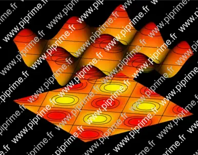
import graph3;
import palette;

real sinc(real x){return x != 0 ? sin(x)/x : 1;}

real f(pair z){
  real value = (sinc(pi*z.x)*sinc(pi*z.y))**2;
  return value^0.25;
}

currentprojection=orthographic(0,0,1);

size(10cm,0);

surface s=surface(f,(-5,-5),(5,5),100,Spline);
s.colors(palette(s.map(zpart),Gradient((int)2^11 ... new pen[]{black,white})));

draw(planeproject(unitsquare3)*s,nolight);
graph3-fig013
From TeXgraph exemples.
Show graph3/fig0130.asy on Github.
Generated with Asymptote 3.00-0.
Categories : Examples 3D | Graph3.asy
Tags : #Graph (3D) | #Palette | #Surface | #Shading (3D)
settings.render=0;
import graph3;
import palette;
size(10cm,0);
currentprojection=orthographic(2,-2,2.5);

real f(pair z) {
  real u=z.x, v=z.y;
  return (u/2+v)/(2+cos(u/2)*sin(v));
}

surface s=surface(f,(0,0),(14,14),150,Spline);
draw(s,mean(palette(s.map(zpart),Gradient(yellow,red))));

if(!is3D())
  shipout(bbox(3mm,Fill(black)));
graph3-fig014
From TeXgraph exemples.
Show graph3/fig0140.asy on Github.
Generated with Asymptote 3.00-0.
Categories : Examples 3D | Graph3.asy
Tags : #Graph (3D) | #Palette | #Surface | #Shading (3D)
settings.render=0;
import graph3;
import palette;
size(15cm,0);
currentprojection=orthographic(2,-2,2.5);

real f(pair z) {
  real u=z.x, v=z.y;
  return (u/2+v)/(2+cos(u/2)*sin(v));
}

surface s=surface(f,(0,0),(14,14),50,Spline);
s.colors(palette(s.map(zpart),Gradient(yellow,red)));

draw(s);

if(!is3D())
  shipout(bbox(3mm,Fill(black)));
graph3-fig015

Show graph3/fig0150.asy on Github.
Generated with Asymptote 3.00-0.
Categories : Examples 3D | Graph3.asy
Tags : #Graph (3D) | #Palette | #Surface | #Shading (3D) | #Array | #Spherical harmonics
settings.render=0;
import graph3;
size(15cm);

currentprojection=orthographic(4,2,4);

real r(real Theta, real Phi){return 1+0.5*(sin(2*Theta)*sin(2*Phi))^2;}
triple f(pair z) {return r(z.x,z.y)*expi(z.x,z.y);}

pen[] pens(triple[] z)
{
  return sequence(new pen(int i) {
      real a=abs(z[i]);
      return a < 1+1e-3 ? black : interp(blue, red, 2*(a-1));
    },z.length);
}

surface s=surface(f,(0,0),(pi,2pi),100,Spline);
// Interpolate the corners, and coloring each patch with one color
// produce some artefacts
draw(s,pens(s.cornermean()));

if(!is3D())
  shipout(bbox(3mm,Fill(black)));
graph3-fig016
Show graph3/fig0160.asy on Github.
Generated with Asymptote 3.00-0.
Categories : Examples 3D | Graph3.asy
Tags : #Graph (3D) | #Palette | #Surface | #Shading (3D) | #Array | #Spherical harmonics
settings.render=0;
import graph3;
size(15cm);

currentprojection=orthographic(4,2,4);

real r(real Theta, real Phi){return 1+0.5*(sin(2*Theta)*sin(2*Phi))^2;}
triple f(pair z) {return r(z.x,z.y)*expi(z.x,z.y);}

pen[][] pens(triple[][] z)
{
  pen[][] p=new pen[z.length][];
  for(int i=0; i < z.length; ++i) {
    triple[] zi=z[i];
    p[i]=sequence(new pen(int j) {
	real a=abs(zi[j]);
	return a < 1+1e-3 ? black : interp(blue, red, 2*(a-1));},
      zi.length);
  }
  return p;
}

surface s=surface(f,(0,0),(pi,2pi),100,Spline);
// Here we interpolate the pens, this looks smoother, with fewer artifacts
draw(s,mean(pens(s.corners())));

if(!is3D())
  shipout(bbox(3mm,Fill(black)));
graph3-fig017
Show graph3/fig0170.asy on Github.
Generated with Asymptote 3.00-0.
Categories : Examples 3D | Graph3.asy
Tags : #Graph (3D) | #Palette | #Surface | #Shading (3D) | #Array | #Spherical harmonics
import graph3;
size(16cm, 0);

currentprojection=orthographic(4, 2, 4);

real r(real Theta, real Phi){return 1+0.5*(sin(2*Theta)*sin(2*Phi))^2;}
triple f(pair z) {return r(z.x, z.y)*expi(z.x, z.y);}

pen[][] pens(triple[][] z)
{
  pen[][] p=new pen[z.length][];
  for(int i=0; i < z.length; ++i) {
    triple[] zi=z[i];
    p[i]=sequence(new pen(int j) {
    real a=abs(zi[j]);

    return a < 1+1e-3 ? black : interp(blue, red, 2*(a-1));}, zi.length);
  }

  return p;
}

surface s=surface(f, (0, 0), (pi, 2pi), 100, Spline);
// Here we determine the colors of vertexes (vertex shading).
// Since the PRC output format does not support vertex shading of Bezier surfaces, PRC patches
// are shaded with the mean of the four vertex colors.
s.colors(pens(s.corners()));
draw(s);

if(!is3D())
  shipout(bbox(1mm, Fill(black)));
graph3-fig018
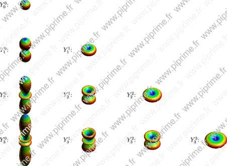
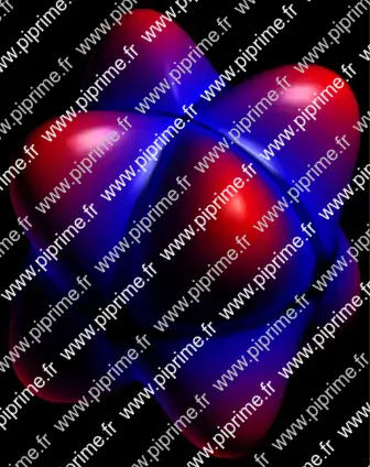
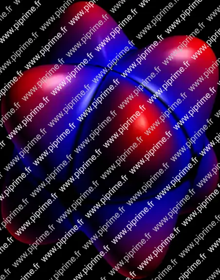
The spherical harmonics are the angular portion of the solution to Laplace's equation in spherical coordinates where azimuthal symmetry is not present.
The spherical harmonics are defined by:
where and is the Legendre polynomial.
Source
Show graph3/fig0180.asy on Github.
Generated with Asymptote 3.00-0.
Categories : Examples 3D | Graph3.asy
Tags : #Graph (3D) | #Palette | #Surface | #Shading (3D) | #Spherical harmonics
import palette;
import math;
import graph3;

typedef real fct(real);
typedef pair zfct2(real,real);
typedef real fct2(real,real);

real binomial(real n, real k)
{
  return gamma(n+1)/(gamma(n-k+1)*gamma(k+1));
}

real factorial(real n) {
  return gamma(n+1);
}

real[] pdiff(real[] p)
{ // p(x)=p[0]+p[1]x+...p[n]x^n
  // retourne la dérivée de p
  real[] dif;
  for (int i : p.keys) {
    if(i != 0) dif.push(i*p[i]);
  }
  return dif;
}

real[] pdiff(real[] p, int n)
{ // p(x)=p[0]+p[1]x+...p[n]x^n
  // dérivée n-ième de p
  real[] dif={0};
  if(n >= p.length) return dif;
  dif=p;
  for (int i=0; i < n; ++i)
    dif=pdiff(dif);
  return dif;
}

fct operator *(real y, fct f)
{
  return new real(real x){return y*f(x);};
}

zfct2 operator +(zfct2 f, zfct2 g)
{// Défini f+g
  return new pair(real t, real p){return f(t,p)+g(t,p);};
}

zfct2 operator -(zfct2 f, zfct2 g)
{// Défini f-g
  return new pair(real t, real p){return f(t,p)-g(t,p);};
}

zfct2 operator /(zfct2 f, real x)
{// Défini f/x
  return new pair(real t, real p){return f(t,p)/x;};
}

zfct2 operator *(real x,zfct2 f)
{// Défini x*f
  return new pair(real t, real p){return x*f(t,p);};
}

fct fct(real[] p)
{ // convertit le tableau des coefs du poly p en fonction polynôme
  return new real(real x){
    real y=0;
    for (int i : p.keys) {
      y += p[i]*x^i;
    }
    return y;
  };
}

real C(int l, int m)
{
  if(m < 0) return 1/C(l,-m);
  real OC=1;
  int d=l-m, s=l+m;
  for (int i=d+1; i <=s ; ++i) OC *= i;
  return 1/OC;
}

int csphase=-1;
fct P(int l, int m)
{ // Polynôme de Legendre associé
  // http://mathworld.wolfram.com/LegendrePolynomial.html
  if(m < 0) return (-1)^(-m)*C(l,-m)*P(l,-m);
  real[] xl2;
  for (int k=0; k <= l; ++k) {
    xl2.push((-1)^(l-k)*binomial(l,k));
    if(k != l) xl2.push(0);
  }
  fct dxl2=fct(pdiff(xl2,l+m));
  return new real(real x){
    return (csphase)^m/(2^l*factorial(l))*(1-x^2)^(m/2)*dxl2(x);
  };
}

zfct2 Y(int l, int m)
{// http://fr.wikipedia.org/wiki/Harmonique_sph%C3%A9rique#Expression_des_harmoniques_sph.C3.A9riques_normalis.C3.A9es
  return new pair(real theta, real phi) {
    return sqrt((2*l+1)*C(l,m)/(4*pi))*P(l,m)(cos(theta))*expi(m*phi);
  };
}

real xyabs(triple z){return abs(xypart(z));}

size(16cm);
currentprojection=orthographic(0,1,1);

zfct2 Ylm;

triple F(pair z)
{
  //   real r=0.75+dot(0.25*I,Ylm(z.x,z.y));
  //   return r*expi(z.x,z.y);
  real r=abs(Ylm(z.x,z.y))^2;
  return r*expi(z.x,z.y);
}

int nb=4;
for (int l=0; l < nb; ++l) {
  for (int m=0; m <= l; ++m) {
    Ylm=Y(l,m);

    surface s=surface(F,(0,0),(pi,2pi),60);
    s.colors(palette(s.map(xyabs),Rainbow()));

    triple v=(-m,0,-l);
    draw(shift(v)*s);
    label("$Y_"+ string(l) + "^" + string(m) + "$:",shift(X/3)*v);
  }
}